Regression: Torch as a Tensor library

回归问题是一种寻找自变量与因变量之间的关系的统计建模方法。

设有自变量 \(\boldsymbol{x}\) 和因变量 \(y\) 符合 \(y = g(\boldsymbol{x})\)，则回归的任务是找到一个 \(f(\cdot)\)，\(\mathrm{s.t.} \min{\mathrm{dist}(f(\boldsymbol x), g(\boldsymbol x))}\)。

较为常用的，也是最简单的，是线性回归模型。虽然单变量线性回归在中学已经学过解析解了

线性回归假设自变量与因变量成线性关系，也就是

\[ H(x) = Wx+b \]

由此关系我们构造 cost function：

\[ \begin{gathered} cost=\frac{1}{m} \sum_{i=1}^{m}\left(H\left(x^{(i)}\right)-y^{(i)}\right)^{2} \\ H(x)=W x+b \end{gathered} \]

其中 \(W\) 和 \(b\) 被称为参数，故也可以写作

\[ \operatorname{cost}(W, b)=\frac{1}{m} \sum_{i=1}^{m}\left(H\left(x^{(i)}\right)-y^{(i)}\right)^{2} \]

目标函数就是：

\[ \min_{W, b} \operatorname{cost}(W, b) \]

读作 Minimize \(\operatorname{cost}(W, b)\) with regard to \(W\) and \(b\).

那么比如我们拿到了_~西瓜~数据

x	Y
1	1
2	2
3	3

对于每对 \((x, Y)\) 我们都可以计算 \(\mathrm{cost}\)。

这里利用 PyTorch 进行计算。

import torch
import numpy as np

def cost(W: torch.Tensor, x: torch.Tensor, y: torch.Tensor) -> torch.Tensor:
    x = x.unsqueeze(-1)
    y = y.unsqueeze(-1)
    return torch.mean(torch.square(W * x - y), (0,))

x = torch.tensor([1., 2., 3.])
y = torch.tensor([1., 2., 3.])

print(cost(W, x, y)) # tensor(4.6667)
W = torch.ones(3)
print(cost(W, x, y)) # tensor(0.)
W = torch.full((3,), 2)
print(cost(W, x, y)) # tensor(4.6667)

# What does cost(W) look like?
%matplotlib inline
import matplotlib.pyplot as plt
rng = torch.arange(-3., 5., 0.01)
inp = torch.stack([rng]*3)

output = cost(inp, x, y)
plt.plot(rng.numpy(), output.numpy())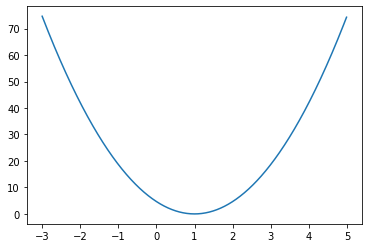

问题是：如何最小化这个损失函数？

解析解是这样的：

\[ \operatorname{cost}(W)=\frac{1}{2 m} \sum_{i=1}^{m}\left(W x^{(i)}-y^{(i)}\right)^{2} \]

则求偏导

\[ \frac{\partial }{\partial W}\mathrm{cost}(W) = \frac{1}{m} \sum_{i=1}^{m} x^{(i)} \left(W x^{(i)}-y^{(i)}\right) \]

虽然这个简单的方程有解析解，但对于大多数优化问题来说是没有解析解的。在此节中我们将学习如何利用梯度下降法求解回归问题。

\[ \begin{gathered} W:=W-\alpha \frac{\partial}{\partial W} \operatorname{cost}(W) \\ W:=W-\alpha \frac{1}{m} \sum_{i=1}^{m}\left(W x^{(i)}-y^{(i)}\right) x^{(i)} \end{gathered} \]

import torch
from torch.utils.data import Dataset, DataLoader
from torch.utils.tensorboard import SummaryWriter
import numpy as np
np.random.seed(42)
import matplotlib.pyplot as plt

class FakeDataset(Dataset):
    def __init__(self):
        super(FakeDataset, self).__init__()
        k = np.random.random()
        self.x = x = np.arange(1, 4)
        b = np.arange(1, 4)
        self.val = k * x + b
        # print("Guess: ", k, b)
        self.data = list(zip(x, k*x+b))

    def __getitem__(self, index):
        return self.data[index]

    def __len__(self):
        return len(self.data);


class Net(torch.nn.Module):
    def __init__(self):
        super(Net, self).__init__()
        self.k = torch.tensor(10000., requires_grad=True)
        self.b = torch.rand(1, requires_grad=True)

    def forward(self, input):
        return input * self.k + self.b

def loss_fn(out, target):
    return (out-target)**2

if __name__ == '__main__':
    dataset = FakeDataset()
    model = Net()
    tb = SummaryWriter(log_dir="runs")

    step = 1
    lr = 0.01
    EPOCHS = 1000
    for epoch in range(1, EPOCHS):
        for x, val in dataset:
            out = model(x)
            loss = loss_fn(out, val)
            model.k.grad = None
            model.b.grad = None
            loss.backward()
            with torch.no_grad():
                tb.add_scalar("Loss", float(loss), step)
                step+=1
                model.k -= lr*model.k.grad
                model.b -= lr*model.b.grad

    plt.scatter(dataset.x, dataset.val)
    eval_out = model(torch.tensor(np.arange(1, 11)))
    plt.plot(np.arange(1, 11), eval_out.detach().numpy())
    plt.show()

---

最后更新: 2023-01-31