Restricted Boltzmann Machine
This is an original article. I write it in English with some hope to practice academic writing.
Boltzmann machine was first introduced in 1985 by Geoffrey Hinton. It is a generative unsupervised model which involves learning a probability distribution.
Boltzmann distribution
The working of Boltzmann Machine is mainly inspired by the Boltzmann distribution, which originates form statistical physics. We don't really care about its derivation, so we present it as
What makes RBMs different from Boltzmann machines is that visible nodes and hidden nodes form the two partitions of a bipartite graph.
- Visible nodes: input data
- Hidden nodes: computed results.
Put it mathematically, values of visible nodes and hidden nodes confront to the Boltzmann distribution. The energy function is defined as
and the normalization term is
(but wait, why it is defined as this?)
We define a joint distribution as
Training
There are two methods to speed up the training procedure: contrastive divergence and persistent contrastive divergence.

This restriction imposed on the connections makes the input and the hidden nodes independent within the layer.
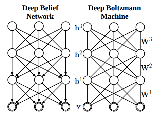
Deep Boltzmann Machines
Deep Boltzmann Machines (DBM)
DBM is often confused with Deep Belief Networks (DBN) as they work in a similar manner.
RBM in PyTorch
import numpy as np
import torch
import torch.utils.data
import torch.nn as nn
import torch.nn.functional as F
import torch.optim as optim
from torch.autograd import Variable
from torchvision import datasets, transforms
from torchvision.utils import make_grid , save_image
import matplotlib.pyplot as plt

# Setup the MNIST dataset

batch_size = 64
train_loader = torch.utils.data.DataLoader(
datasets.MNIST('./data',
    train=True,
    download = True,
    transform = transforms.Compose(
        [transforms.ToTensor()])
     ),
     batch_size=batch_size
)

test_loader = torch.utils.data.DataLoader(
datasets.MNIST('./data',
    train=False,
    transform=transforms.Compose(
    [transforms.ToTensor()])
    ),
    batch_size=batch_size)

class RBM(nn.Module):
   def __init__(self,
               n_vis=784,
               n_hin=500,
               k=5):
        super(RBM, self).__init__()
        self.W = nn.Parameter(torch.randn(n_hin,n_vis)*1e-2)
        self.v_bias = nn.Parameter(torch.zeros(n_vis))
        self.h_bias = nn.Parameter(torch.zeros(n_hin))
        self.k = k

   def sample_from_p(self,p):
       return F.relu(torch.sign(p - Variable(torch.rand(p.size()))))

   def v_to_h(self,v):
        p_h = F.sigmoid(F.linear(v,self.W,self.h_bias))
        sample_h = self.sample_from_p(p_h)
        return p_h,sample_h

   def h_to_v(self,h):
        p_v = F.sigmoid(F.linear(h,self.W.t(),self.v_bias))
        sample_v = self.sample_from_p(p_v)
        return p_v,sample_v

   def forward(self,v):
        pre_h1,h1 = self.v_to_h(v)

        h_ = h1
        for _ in range(self.k):
            pre_v_,v_ = self.h_to_v(h_)
            pre_h_,h_ = self.v_to_h(v_)

        return v,v_

   def free_energy(self,v):
        vbias_term = v.mv(self.v_bias)
        wx_b = F.linear(v,self.W,self.h_bias)
        hidden_term = wx_b.exp().add(1).log().sum(1)
        return (-hidden_term - vbias_term).mean()

rbm = RBM(k=1)
train_op = optim.SGD(rbm.parameters(),0.1)

for epoch in range(10):
    loss_ = []
    for _, (data,target) in enumerate(train_loader):
        data = Variable(data.view(-1,784))
        sample_data = data.bernoulli()

        v,v1 = rbm(sample_data)
        loss = rbm.free_energy(v) - rbm.free_energy(v1)
        loss_.append(loss.data)
        train_op.zero_grad()
        loss.backward()
        train_op.step()

    print("Training loss for {} epoch: {}".format(epoch, np.mean(loss_)))

def show_and_save(file_name,img):
    npimg = np.transpose(img.numpy(),(1,2,0))
    f = "./%s.png" % file_name
    plt.imshow(npimg)
    plt.imsave(f,npimg)

show_and_save("real",make_grid(v.view(32,1,28,28).data))
show_and_save("generate",make_grid(v1.view(32,1,28,28).data))