Tech Report

在 COCO 2014 数据集上训练 AoAnet¶

基于AoAnet进行训练，参考文献：https://arxiv.org/abs/1908.06954

@inproceedings{huang2019attention,
  title={Attention on Attention for Image Captioning},
  author={Huang, Lun and Wang, Wenmin and Chen, Jie and Wei, Xiao-Yong},
  booktitle={International Conference on Computer Vision},
  year={2019}
}

数据¶

数据集的下载¶

COCO 图片¶

项目需要 COCO 2014 数据集的 train 和 val，可以从官网下载：

wget -c http://images.cocodataset.org/zips/train2014.zip http://images.cocodataset.org/annotations/image_info_val2014.zip

全部链接：

http://images.cocodataset.org/zips/train2014.zip

http://images.cocodataset.org/annotations/annotations_trainval2014.zip

http://images.cocodataset.org/zips/val2014.zip

http://images.cocodataset.org/annotations/image_info_val2014.zip

http://images.cocodataset.org/zips/test2014.zip

http://images.cocodataset.org/annotations/image_info_test2014.zip

也可以通过 Redmon 的镜像站：https://pjreddie.com/projects/coco-mirror/

注意train2014中有一张图像坏掉了，需要替换，参考，替换方式：

cd train2014
curl https://msvocds.blob.core.windows.net/images/262993_z.jpg >> COCO_train2014_000000167126.jpg

预处理后的描述¶

wget http://cs.stanford.edu/people/karpathy/deepimagesent/caption_datasets.zip

代码仓库¶

git clone https://github.com/husthuaan/AoANet.git --recursive

注意两个submodule是不是都下载下来了。

数据预处理¶

预处理标注¶

下面这个预处理需要python2的环境，搭建环境：

conda create -n py2 python<3
conda activate py2
conda install pytorch cpuonly -c pytorch
conda install six

python scripts/prepro_ngrams.py --input_json data/dataset_coco.json --dict_json data/cocotalk.json --output_pkl data/coco-train --split train

本项目使用 ResNet 提取特征，预处理流程如下。

下载模型：

curl https://download.pytorch.org/models/resnet101-63fe2227.pth >> ./data/imagenet_weights/resnet101.pth

创建环境，此处使用docker

# docker-compose.yml
version: "3"
services:
  pytorch:
    image: "ufoym/deepo:pytorch-cu111"
    ports:
      - "0:22"
    volumes:
      - $HOME:$HOME
      - /nvme:/nvme
      # 记得把代码所在目录映射进来
    shm_size: "32gb"
    deploy:
      resources:
        reservations:
          devices:
            - capabilities: ["gpu"]

docker-compose up -d
docker exec -it AoAnet_pytorch bash # 进入容器
cd # 代码所在目录
pip install h5py yacs lmdbdict pyemd
export PYTHONPATH=`pwd`

然后就可以开始进行预处理

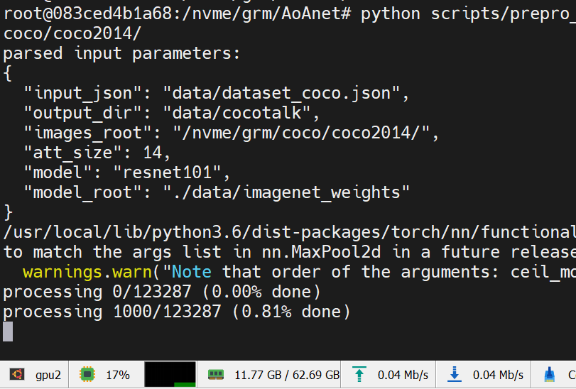
python scripts/prepro_labels.py --input_json data/dataset_coco.json --output_json data/cocotalk.json --output_h5 data/cocotalk

python scripts/prepro_feats.py --input_json data/dataset_coco.json --output_dir data/cocotalk --images_root $IMAGE_ROOT

预处理速度很慢，耐心等待

在训练时遇到了问题，没库，没依赖，作者也不提供一下参考

sudo apt install openjdk-8-jdk # 依赖
pip install gensim # NLP库

# 下载Word2Vec的一个模型
cd coco-caption/pycocoevalcap/wmd/data
wget -c "https://s3.amazonaws.com/dl4j-distribution/GoogleNews-vectors-negative300.bin.gz"
gzip -d GoogleNews-vectors-negative300.bin.gz

from gensim import models
w = models.KeyedVectors.load_word2vec_format('./GoogleNews-vectors-negative300.bin', binary=True)

作者怎么不把依赖写全，非要等到跑到一个 epoch 结束扔个异常出来。气。抓异常只抓(RuntimeError, KeyboardInterrupt)，您就没考虑过有人可能没装全依赖吗。

注意还有一处调用torch.optim.lr_scheduler.ReduceLROnPlateau()参数顺序因PyTorch版本调整有所改变，需要将verbose参数移到最后。

torch.optim.lr_scheduler.ReduceLROnPlateau(optimizer, mode='min', factor=0.1, patience=10, threshold=0.0001, threshold_mode='rel', cooldown=0, min_lr=0, eps=1e-08, verbose=False)

使用 ResNet feature¶

python scripts/prepro_feats.py --input_json data/dataset_coco.json --output_dir data/cocotalk --images_root $IMAGE_ROOT

使用 ResNet feature 训练，需要修改train.sh中的配置使目录指向 cocotalk 目录。实测 25 epoch 指标：

Bleu_1: 0.724
Bleu_2: 0.551
Bleu_3: 0.405
Bleu_4: 0.295
METEOR: 0.250
ROUGE_L: 0.530
CIDEr: 0.954
SPICE: 0.182
WMD: 0.533

指标并不能达到论文中的高度，怀疑是数据使用出了问题。论文中使用的 feature 是 bottom-up feature，

使用 Bottom-Up feature¶

Download pre-extracted feature from link. You can either download adaptive one or fixed one.

下载方式如下：

mkdir data/bu_data; cd data/bu_data
wget https://storage.googleapis.com/up-down-attention/trainval.zip
unzip trainval.zip
# 切回项目根目录
cd ..
conda acitivate py2 # python2文件，因为reader迭代器返回了byte
python scripts/make_bu_data.py --output_dir data/cocobu

然后我把train.sh改了回去(git checkout train.sh)，备份了checkpoints，清理项目目录，重新开始训练。

CUDA_VISIBLE_DEVICES=0 bash train.sh

所有训练选项：

Namespace(
    acc_steps=1,
    att_feat_size=2048,
    att_hid_size=512,
    batch_size=16,
    beam_size=1,
    bleu_reward_weight=0,
    block_trigrams=0,
    cached_tokens='coco-train-idxs',
    caption_model='aoa',
    checkpoint_path='log/log_aoanet',
    cider_reward_weight=1,
    ctx_drop=1,
    decoder_type='AoA',
    drop_prob_lm=0.5,
    dropout_aoa=0.3,
    fc_feat_size=2048,
    grad_clip=0.1,
    id='aoanet',
    input_att_dir='data/cocobu_att',
    input_box_dir='data/cocobu_box',
    input_encoding_size=1024,
    input_fc_dir='data/cocobu_fc',
    input_json='data/cocotalk.json',
    input_label_h5='data/cocotalk_label.h5',
    label_smoothing=0.2,
    language_eval=1,
    learning_rate=0.0002,
    learning_rate_decay_every=3,
    learning_rate_decay_rate=0.8,
    learning_rate_decay_start=0,
    length_penalty='',
    load_best_score=1,
    logit_layers=1,
    losses_log_every=25,
    max_epochs=50,
    max_length=20,
    mean_feats=1,
    multi_head_scale=1,
    noamopt=False,
    noamopt_factor=1,
    noamopt_warmup=2000,
    norm_att_feat=0,
    norm_box_feat=0,
    num_heads=8,
    num_layers=2,
    optim='adam',
    optim_alpha=0.9,
    optim_beta=0.999,
    optim_epsilon=1e-08,
    reduce_on_plateau=False,
    refine=1,
    refine_aoa=1,
    remove_bad_endings=0,
    rnn_size=1024,
    rnn_type='lstm',
    save_checkpoint_every=6000,
    save_history_ckpt=0,
    scheduled_sampling_increase_every=5,
    scheduled_sampling_increase_prob=0.05,
    scheduled_sampling_max_prob=0.5,
    scheduled_sampling_start=0,
    self_critical_after=-1,
    seq_length=16,
    seq_per_img=5,
    start_from='log/log_aoanet',
    train_only=0,
    use_att=True,
    use_bn=0,
    use_box=0,
    use_fc=True,
    use_ff=0,
    use_multi_head=2,
    use_warmup=0,
    val_images_use=-1,
    vocab_size=9487,
    weight_decay=0
)

注意使用nohup时需要使用2) SIGINT打断（kill默认发送的是15) SIGTERM），

kill -2 $pid # 注意要打断python父程序（pid最小的那个）而不是启动脚本用的bash！

注意由于PyTorch 1.5中BiLSTM模块更新导致pack_padded_sequence的length只能是CPU int64 tensor，参考 ISSUE 43227，之前的版本会将length隐式复制到内存，所以后来PyTorch废弃了这种写法。

我们需要修改models/AttModel.py中sort_pack_padded_sequence函数如下：

def sort_pack_padded_sequence(input, lengths):
    sorted_lengths, indices = torch.sort(lengths, descending=True)
    # 修改下一行，加入.cpu()
    tmp = pack_padded_sequence(input[indices], sorted_lengths.cpu(), batch_first=True)
    inv_ix = indices.clone()
    inv_ix[indices] = torch.arange(0,len(indices)).type_as(inv_ix)
    return tmp, inv_ix

另外，半年之后，PaddlePaddle还是没有pack_padded_sequence这个 API，可能需要自己写。参照：https://www.paddlepaddle.org.cn/documentation/docs/faq/train_cn.html#paddletorch-nn-utils-rnn-pack-padded-sequencetorch-nn-utils-rnn-pad-packed-sequenceapi

测试指标¶

本次使用五个指标：Bleu、METEOR、ROUGE-L、CIDEr、SPICE。

目标指标如下：

{
    ‘Bleu_1’: 0.8054903453672397,
    ‘Bleu_2’: 0.6523038976984842,
    ‘Bleu_3’: 0.5096621263772566,
    ‘Bleu_4’: 0.39140307771618477,
    ‘METEOR’: 0.29011216375635934,
    ‘ROUGE_L’: 0.5890369750273199,
    ‘CIDEr’: 1.2892294296245852,
    ‘SPICE’: 0.22680092759866174
}

Perplexity¶

\[ \log_2\operatorname{PPL}(w_{1:L}|I) = -\frac{1}{L}\sum_{n=1}^L(\log_2\operatorname{P}(w_n | w_{1:n-1}, I)) \]

其中，\(L\)是句子的长度，\(\operatorname{PPL}(w_{1:L},I)\)是根据图像\(I\)给出的描述句子\(w_{1:L}\)的\(\operatorname{preplexity}\)，而\(\operatorname{P}(w_n | w_{1:n-1}, I)\)是根据图像\(I\)和前\(n-1\)个单词组成的序列生成下一个单词\(w_n\)的概率。

\(\operatorname{preplexity}\)用于判断模型的稳定性，得分越低就认为模型的预测越稳定，翻译质量越好。

Bleu¶

Bilingual Evaluation Underatudy，用于分析候选译文和参考译文中\(N\)元组共同出现的程度，重合程度越高就认为译文质量越高。

\[ \operatorname{BLEU} = BP \times \exp\left(\sum_{n=1}^N w_n \log P_n \right) \]

\(BP\)表示短句子的惩罚因子（Brevity Penalty），用\(l_r\)表示最短的参考翻译的长度，\(l_c\)表示候选翻译的长度，具体计算方法：

\[ BP = \begin{cases} 1 & l_c > l_s \\ \mathrm{e}^{1-\frac{l_s}{l_c}} & l_c \le l_s \end{cases} \]

\(P(n)\)表示 n-gram 的覆盖率，计算方式为：

\[ p_{n}=\frac{\sum_{C \in\{\text { Candidates }\}} \sum_{\text { n-gram } \in C} \text { Count }_{\text {clip }}(\text { n-gram })}{\sum_{C^{\prime} \in\{\text { Candidates }\}} \sum_{\text { n-gram } \in C^{\prime}} \text { Count }(\text { n-gram })} \]

其中\(\text{Count}_{\text{clip}}\)是截断技术，其计数方式为：将一个 n-gram 在候选翻译中出现的次数，与在各个参考翻译中出现次数的最大值进行比较，取较小的那一个。

METEOR¶

Metric for Evaluation of Translation with Explicit ORdering 基于 BLEU 进行了一些改进，使用 WordNet 计算特有的序列匹配、同义词、词根和词缀，以及释义之间的匹配关系。

\[ \operatorname{METEOR} = (1-Pen) \times F_{\text{means}} \]

其中\(Pen = \frac{\#chucks}{m}\)为惩罚因子，惩罚候选翻译中词序与参考翻译中次词序的不同。

\[ F_\text{meams} = \frac{PR}{\alpha P + (1-\alpha)R} \]

其中\(\alpha\)为超参数，\(P=\frac{m}{c}\)，\(R = \frac{m}{r}\)，\(m\)为候选翻译中能够被匹配的一元组的数量，\(c\)为候选翻译的长度，\(r\)为参考翻译的长度。

METEOR 基于准确率和召回率，得分越高说明

ROUGE¶

Recall-Oriented Understudy for Gisting Evaluation，大致分为四种：ROUGE-N，ROUGE-L，ROUGE-W，ROUGE-S。

\[ \operatorname{ROUGE-N}=\frac{\sum_{S \in\{\text { ReferenceSummaries }\}} \sum_{\text {gram }_{n} \in S} \text { Count }_{\text {match }}\left(\text { gram }_{n}\right)}{\sum_{S \in\{\text { ReferenceSummaries }\}} \sum_{\text {gram }_{n} \in S} \text { Count }\left(\text { gram }_{n}\right)} \]

其中\(n\)表示 n-gram，\(\text{Count}{(\text{gram}_n)}\)表示一个 n-gram 出现的次数，\(\text{Count}_{\text{match}}{(\text{gram}_n)}\)表示一个 n-gram 共现的次数。

\[ \begin{aligned} \operatorname{ROUGE-L} &=\frac{\left(1+\beta^{2}\right) R_{l c s} P_{l c s}}{R_{l c s}+\beta^{2} P_{l c s}} \\ R_{l c s} &=\frac{\operatorname{LCS}(X, Y)}{m} \\ P_{l c s} &=\frac{\operatorname{LCS}(X, Y)}{n} \end{aligned} \]

其中，\(X\)表示候选摘要，\(Y\)表示参考摘要，\(\operatorname{LCS}\)表示候选摘要与参考摘要的最长公共子序列的长度，\(m\)表示参考摘要的长度，\(n\)表示候选摘要的长度。

CIDEr¶

Consensus-based Image Description Evaluation 将每个句子看成文档，计算其 Term Frequency Inverse Document Frequency（TF-IDF）向量的余弦夹角，据此得到候选句子和参考句子的相似程度。

\[ \operatorname{CIDEr}_n(c, S) = \frac{1}{M} \sum_{i=1}^M \frac{g^n(c)\cdot g^n\left(S_i\right)}{||g^n(c)|| \times ||g^n\left(S_i\right)||} \]

其中\(c\)表示候选标题，\(S\)表示参考标题集合，\(n\)表示评估的是 n-gram，M 表示标题的数量，\(g^n(\cdot)\)表示基于 n-gram 的 TF-IDF 向量。

\[ \operatorname{CIDEr}\left(c_{i}, S_{i}\right)=\sum_{n=1}^{N} w_{n} \operatorname{CIDEr}_{n}\left(c_{i}, S_{i}\right) \]

TF-IDF 的计算方式为：

\[ g_{k}\left(s_{i j}\right)=\frac{h_{k}\left(s_{i j}\right)}{\sum_{\omega_{l} \in \Omega} h_{l}\left(s_{i j}\right)} \log \left(\frac{|I|}{\sum_{I_{p} \in I} \min \left\{1, \sum_{q} h_{k}\left(s_{p q}\right)\right\}}\right) \]

SPICE¶

Semantic Propositional Image Caption Evaluation 使用基于图的语义表示来编码 caption 中的 objects，attributes 和 relationships。它先将待评价 caption 和参考 captions 用 Probabilistic Context-Free Grammar (PCFG) dependency parser parse 成 syntactic dependencies trees，然后用基于规则的方法把 dependency tree 映射成 scene graphs。最后计算待评价的 caption 中 objects, attributes 和 relationships 的 F-score 值。

\[ \begin{aligned} \operatorname{SPICE}(c, S) &=F_{1}(c, S)=\frac{2 \cdot P(c, S) \cdot R(c, S)}{P(c, S)+R(c, S)} \\ P(c, S) &=\frac{|T(G(c)) \otimes T(G(S))|}{|T(G(c))|} \\ R(c, S) &=\frac{|T(G(c)) \otimes T(G(S))|}{|T(G(S))|} \end{aligned} \]

其中，\(c\)表示候选标题，\(S\)表示参考标题集合，\(G(\cdot)\)表示利用某种方法将一段文本转化为一个 Scene Graph，\(T(\cdot)\)表示将一个 Scene Graph 转换为一个 Tuple 的集合。\(\otimes\)运算类似于交集，但其匹配类似于 METEOR 中的基于 WordNet 的匹配。

WMD¶

Word Mover’s Distance³

算法分析¶

Attention 机制¶

Encoder¶

设\((h_1, h_2, \ldots, h_n)\)是输入句子的隐藏向量表示。这些向量可以是一个 bi-LSTM 的输出，可以捕捉每个词在剧中的语义信息。

Decoder¶

设第\(i\)个 decoder 的 hidden state 是\(s_i\)，使用一个递归公式计算：

\[ s_i = f(s_{i-1}, y_{i-1}, c_i) \]

其中，\(s_{i-1}\)是上一个隐藏向量，\(y_{i-1}\)是上一步生成的词向量，\(c_i\)是上下文信息。

\[ e_{i, j} = a(s_{i-1}, h_j) \]

其中\(a\)可以是任何函数，通常采用一个前馈神经网络。

最终，对分数正则化：

\[ a_{i, j} = \frac{\exp(e_{i, j})}{\sum_{k=1}^n \exp(e_{i, k})} \]

最终计算\(c_i\)，一个\(h_j\)的加权平均

\[ c_i = \sum_{j=1}^n a_{i, j} h_j \]

或者，一个向量化的表示：

\[ \text { Attention }(Q, K, V)=\operatorname{softmax}\left(\frac{Q K^{T}}{\sqrt{d_{k}}}\right) V \]

Self-Critical Sequence Training⁴¶

REINFORCE 方法¶

在之前，NLP 问题经常使用交叉熵损失函数来优化指标，这有两个不足：一是不能直接优化 NLP 指标，如 CIDEr 等；二是会引起“偏置爆炸”情况。不能直接优化 CIDEr 是因为 CIDEr 的指标是离散的，无法求取梯度。在⁴中将 LSTM 模型视为 agent，将单词和 feature 视作 environment。LSTM 网络的参数，\(\theta\)，定义了一个 policy \(p_\theta\)；其 state 就是它的 cells 和 hidden state。其 action 就是预测下一个单词。每个 action 之后，agent 更新其内部的 state。当模型输出 End-Of-Sequence 后，agent 观测到一个 reward，这个 reward 就可以是生成的句子的 CIDEr 得分。目标是最小化负的 reward 期望

\[ L(\theta) = - \mathbb{E}_{w^s \sim p_\theta}[r(w^s)], \]

\(w^w = (w_1^s, \ldots, w_T^s)\)，\(w_t^s\)是在时间\(t\)从模型中采样出的单词。实际中，通常用\(p_\theta\)中的一个采样估计\(L(\theta)\)。

\[ L(\theta) \approx -r(w^s),\, w^s \sim p_\theta \]

使用 REINFORCE 方法计算不可微的 reward function 的梯度：

\[ \grad_\theta L(\theta) = - \mathbb{E}_{w^s \sim p_\theta}[r(w^s)\grad_\theta \log p_\theta(w^s)]. \]

在实际中，我们从\(p_\theta\)中随机采样\(w^s = (w_1^s, \ldots, w_T^s)\)

\[ \grad_\theta L(\theta) = - r(w^s)\grad_\theta \log p_\theta(w^s). \]

class LanguageModelCriterion(nn.Module):
    def __init__(self):
        super(LanguageModelCriterion, self).__init__()

    def forward(self, input, target, mask):
        # truncate to the same size
        target = target[:, :input.size(1)]
        mask =  mask[:, :input.size(1)]

        output = -input.gather(2, target.unsqueeze(2)).squeeze(2) * mask
        output = torch.sum(output) / torch.sum(mask)

        return output

Bottom-Up feature⁵¶

文献⁵将图像描述生成分成两个任务：一个基于非视觉的或任务上下文驱动的 Attention 机制，命名为 top-down；一个基于纯前馈视觉感知，命名为 bottom-up。文中使用 ResNet101-FasterRCNN 提取 ROI 的 feature vector，将其加权求和得到 bottom-up feature。

AoAnet 论文中训练使用的就是该文献作者提供的 COCO 2014 feature。

AoAnet¶

AoA 机制¶

遵从文献⁶中的表述，记\(f_{att}(\boldsymbol{Q}, \boldsymbol K, \boldsymbol V)\)为一个 Attention 操作。

作者提出使用 AoA 模块计算 attention 结果和 query 的相关性。AoA 模块生成通过两个独立的线性变化生成 information vector \(i\) 和 attention gate \(g\)

\[ \begin{gathered} \boldsymbol{i}=W_{q}^{i} \boldsymbol{q}+W_{v}^{i} \hat{\boldsymbol{v}}+b^{i} \\ \boldsymbol{g}=\sigma\left(W_{q}^{g} \boldsymbol{q}+W_{v}^{g} \hat{\boldsymbol{v}}+b^{g}\right) \end{gathered} \]

where \(W_{q}^{i}, W_{v}^{i}, W_{q}^{g}, W_{v}^{g} \in \mathbb{R}^{D \times D}, b^{i}, b^{g} \in \mathbb{R}^{D}\)，\(D\)是\(\boldsymbol q\)和\(\boldsymbol v\)的维度，\(\hat{\boldsymbol{v}}=f_{a t t}(\boldsymbol{Q}, \boldsymbol{K}, \boldsymbol{V})\)是 Attention 的结果，\(\sigma\)表示 sigmoid 激活函数。

紧接着，AoA 又增加了一层 Attention

\[ \hat{i}=g \odot i \]

整个操作的公式为：

\[ \begin{array}{r} \operatorname{AoA}\left(f_{a t t}, \boldsymbol{Q}, \boldsymbol{K}, \boldsymbol{V}\right)=\sigma\left(W_{q}^{g} \boldsymbol{Q}+W_{v}^{g} f_{a t t}(\boldsymbol{Q}, \boldsymbol{K}, \boldsymbol{V})+b^{g}\right) \\ \odot\left(W_{q}^{i} \boldsymbol{Q}+W_{v}^{i} f_{a t t}(\boldsymbol{Q}, \boldsymbol{K}, \boldsymbol{V})+b^{i}\right) \end{array} \]

实现就是一层的事：

 if self.decoder_type == 'AoA':
     # AoA layer
     self.att2ctx = nn.Sequential(nn.Linear(self.d_model * opt.multi_head_scale + opt.rnn_size, 2 * opt.rnn_size), nn.GLU())

Encoder¶

首先，利用 bottom-up features，每张图片有若干 feature \(\boldsymbol A = \{ \boldsymbol a_1, \boldsymbol a_2, \ldots, \boldsymbol a_k\}\) ， \(\boldsymbol a_i \in \mathbb{R}^D\) 。 \(\boldsymbol A\) 将被送入 AoA refiner 中，通过一个 MultiHeadAttention，外加跳跃连接，最终经过 LayerNorm。

\[ \boldsymbol{A}^{\prime}=\operatorname{LayerNorm}(\boldsymbol{A}+ \left.\operatorname{AoA}^{E}\left(f_{m h-a t t}, W^{Q_{e}} \boldsymbol{A}, W^{K_{e}} \boldsymbol{A}, W^{V_{e}} \boldsymbol{A}\right)\right) \]

\[ \boldsymbol A \leftarrow \boldsymbol A' \]

Decoder¶

与 LSTM 中的 decoder 类似，同样采用一个表征上下文信息的 vector \(\boldsymbol c\)计算下一个词的条件概率：

\[ p\left(\boldsymbol{y}_{t} \mid \boldsymbol{y}_{1: t-1}, I\right)=\operatorname{softmax}\left(W_{p} \boldsymbol{c}_{t}\right) \]

\(W_P\)是权重矩阵，\(|\Sigma{}|\)是词汇量。

\[ \begin{aligned} \boldsymbol{x}_{t} &=\left[W_{e} \Pi_{t}, \overline{\boldsymbol{a}}+\boldsymbol{c}_{t-1}\right] \\ \boldsymbol{h}_{t}, \boldsymbol{m}_{t} &=\operatorname{LSTM}\left(\boldsymbol{x}_{t}, \boldsymbol{h}_{t-1}, \boldsymbol{m}_{t-1}\right) \end{aligned} \]

where \(\bar{\boldsymbol{a}}=\frac{1}{k} \sum_{i} \boldsymbol{a}_{i}\)， \(\boldsymbol c_{-1} = 0\)，\(\boldsymbol c_t\)由以下公式计算得到

\[ \boldsymbol{c}_{t}=\operatorname{AoA}^{D}\left(f_{m h-a t t}, W^{Q_{d}}\left[\boldsymbol{h}_{t}\right], W^{K_{d}} A, W^{V_{d}} A\right) \]

Training & Objective¶

在文献中，前 25 epoch 使用交叉熵损失

\[ L_{X E}(\theta)=-\sum_{t=1}^{T} \log \left(p_{\theta}\left(\boldsymbol{y}_{t}^{*} \mid \boldsymbol{y}_{1: t-1}^{*}\right)\right) \]

紧接着的 40 epoch 使用 Self-Critical Sequence Training，对 CIDEr 进行调优

\[ \nabla_{\theta} L_{R L}(\theta) \approx-\left(r\left(\boldsymbol{y}_{1: T}^{s}\right)-r\left(\hat{\boldsymbol{y}}_{1: T}\right)\right) \nabla_{\theta} \log p_{\theta}\left(\boldsymbol{y}_{1: T}^{s}\right) \]

模型分析¶

类图¶

classDiagram
    class AoAModel {
        use_mean_feats=1
        use_multi_head=2
        ctx2att: AoA
        refiner: AoA_Refiner_Core
        core: AoA_Decoder_Core
        __init__(opt)
        _prepare_feature(fc_feats, att_feats, att_masks) (mean_feats, att_feats, p_att_feats, att_masks)
    }
    class AttModel {
        embed: [Embedding, ReLU, Dropout]
        fc_embed: [Embedding, ReLU, Dropout]
        att_embed: [Embedding, ReLU, Dropout]
        logit: Linear
        vocab: [bad endings, such as 'a', 'the', and so on.]

        __init__(opt)
        init_hidden(batch_size) state
        clip_att(att_feats, att_masks) (att_feats, att_masks)
        _prepare_feature(fc_feats, att_feats, att_masks) (mean_feats, att_feats, p_att_feats, att_masks)
        _forward(fc_feats, att_feats, seq, att_masks=None) outputs
        get_logprobs_state(it, fc_feats, att_feats, p_att_feats, att_masks, state) (logprobs, state)
        _sample_beam(fc_feats, att_feats, att_masks=None, opt=dict()) (deq, seqLogprobs)
        _sample(fc_feats, att_feats, att_masks, opt=dict()) (seq, seqLogprobs)
    }
    class CaptionModel {
        forward(*args, **kwargs) outputs
        beam_search(init_state, init_logprobs, *args, **kwargs) done_beams
        beam_step(logprobsf, unaug_logprobsf, beam_size, t, beam_seq, beam_seq_logprobs, beam_seq_logprobs_sum, state) (beam_seq, beam_seq_logprobs, beam_logprobs_sum, state, candidates)
        sample_next_word(logprobs, sample_method, temprature) (it, sampleLogprobs)
    }
    class AoA_Refiner_Core {
        layer: ModuleList(AoA_Refiner_Layer * 6)
    }
    class AoA_Refiner_Layer {
        self_attn: MultiHeadedDotAttention
        feed_forward: PositionwiseFeedForward
        sublayer: [SublayerConnection]
    }
    class MultiHeadedDotAttention {
        d_k
        h
        project_k_v
        norm: LayerNorm
        linears: [Linear] * [1+2*project_k_v]
        aoa_layer: [Linear, GLU]
        outout_layer: lambda x:x
        dropout
        forward(query, value, key)
    }
    class PositionwiseFeedForward {
        w_1: Linear
        w_2: Linear
        dropout: Dropout
        forward(x)
    }
    class SublayerConnection {
        norm: LayerNorm
        dropout: Dropout
        forward(x, sublayer)
    }
    class AoA_Decoder_Core {
        att2ctx: AoA
        attention: MultiHeadedDotAttention
        ctx_drop: Dropout
        forward(xt, xt, mean_feats, att_feats, p_att_feats, state, att_mask=None) (output, state)
    }
    class TransformerModel {
        ...ommitted
    }
    AoA_Refiner_Core "1"*--"6" AoA_Refiner_Layer
    %% MultiHeadedDotAttention --* AoA_Refiner_Layer
    AoA_Decoder_Core "1"*--"1" MultiHeadedDotAttention
    AoA_Refiner_Layer "1"*--"1" MultiHeadedDotAttention
    AoA_Refiner_Layer "1"*--"1" PositionwiseFeedForward
    AoA_Refiner_Layer "1"*--"2" SublayerConnection

    %% AoA_Refiner_Layer *-- AoA_Refiner_Core
    CaptionModel <|-- AttModel
    AttModel <|-- AoAModel
    AttModel <|-- TransformerModel
    AoAModel *-- AoA_Refiner_Core
    AoAModel *-- AoA_Decoder_Core

论文复现心得¶

要看 README，要多找代码资料，最好是找到有人成功复现了的
复现前的模型通常有各种参数，甚至会有根据参数动态调整网络结构的情况，这种情况下第一步是裁剪，裁剪后看精度能否保持
若第二步成功，那么下一步才是不同框架之间的抹平 API 差异

https://zhuanlan.zhihu.com/p/108630305 ↩
https://www.jianshu.com/p/60deff0f64e1 ↩
https://mkusner.github.io/publications/WMD.pdf ↩
Rennie S J , Marcheret E , Mroueh Y , et al. Self-critical Sequence Training for Image Captioning[J]. IEEE, 2016. https://ieeexplore.ieee.org/document/8099614 ↩↩
Anderson P , He X , Buehler C , et al. Bottom-Up and Top-Down Attention for Image Captioning and Visual Question Answering[C]// 2018 IEEE/CVF Conference on Computer Vision and Pattern Recognition (CVPR). IEEE, 2018. https://ieeexplore.ieee.org/document/8578734 ↩↩
Huang, L. , Wang, W. , Chen, J. , & Wei, X. Y. . Attention on Attention for Image Captioning. International Conference on Computer Vision. Peking University; Peng Cheng Laboratory. https://ieeexplore.ieee.org/document/9008770 ↩

最后更新: 2023-01-31

在 COCO 2014 数据集上训练 AoAnet¶

数据¶

数据集的下载¶

COCO 图片¶

预处理后的描述¶

代码仓库¶

数据预处理¶

预处理标注¶

使用 ResNet feature¶

使用 Bottom-Up feature¶

测试指标¶

Perplexity¶

Bleu¶

METEOR¶

ROUGE¶

CIDEr¶

SPICE¶

WMD¶

算法分析¶

Attention 机制¶

Encoder¶

Decoder¶

Self-Critical Sequence Training4¶

REINFORCE 方法¶

Bottom-Up feature5¶

AoAnet¶

AoA 机制¶

Encoder¶

Decoder¶

Training & Objective¶

模型分析¶

类图¶

论文复现心得¶

Self-Critical Sequence Training⁴¶

Bottom-Up feature⁵¶