ELSA

Self-Attention 擅长捕捉长距离（或者说全局）依赖，但其对局部、细粒度的特征捕捉能力有限。

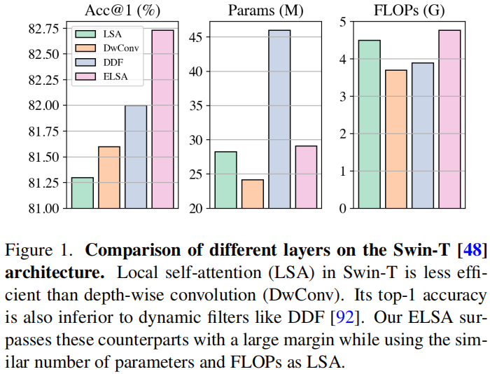
LSA 刚刚能达到卷积的能力，却赶不上 dynamic filters。

Self-Attention 在视觉领域大获成功的背后，Multihead Self Attention 扮演着至关重要的角色。

最近的研究发现 MHSA 倾向于关注在 ViT 前几层的局部信息，所以许多方法试图引入 Inductive Bias 来强制前几层学习局部细节。Swin Transformer 在这方面取得了很大的突破。

但是，奇怪的是，使用 depth-wise convolution 取代 local self-attention 也能取得相媲美（甚至更好）的成绩，并且 LSA 的 FLOPs 更大。

就此，作者提出了文章的核心问题：what makes local self-attention mediocre?

作者首先从 local self-attention、depth-wise convolution 和 dynamic filters 的不同点谈起。

现在在 Vision Transformer 领域公认的是将 Channel 和 Spacial 分开讨论，这篇文章也不例外。

通道设置¶

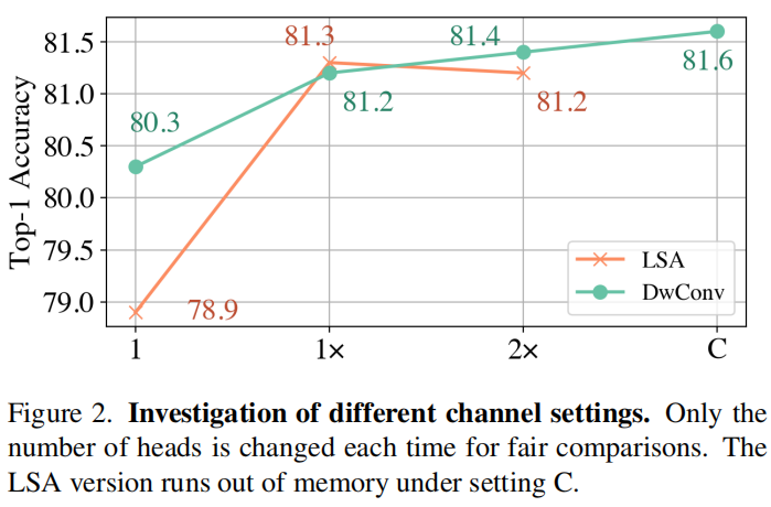
DwConv 和 LSA 最直观的区别在通道设置上。LSA 在一组通道之间共享 filter，但 DwConv 对每个通道使用一个单独的 filter。作者认为 DwConv 是当每组通道里只有一个通道的 LSA，也就是一种 LSA 的特殊情况，进而猜想增加的 Attention Head 数造成是 DwConv 优异表现的关键。但是，经过作者尝试增加 LSA 的头数等于通道数（虽然没有加到，显存不足，见原文 Figure 2），还是表现齐平，或者 DwConv 略胜一筹，并且直接增加 LSA 头数不会提升其表现。

空间处理¶

DwConv 在每个 feature pixel 中以滑动窗口的方式共享一个静态的 filter，Dynamic Filters 使用一个 bypass network（通常是\(1\times 1\)卷积）对一个像素生成一个空间相关的 filter，再把这个 filter 应用到该像素的邻域上。按这个逻辑范式，LSA 使用 \(qurey\) 和 \(key\) 矩阵的点乘生成的 attention map 也可以看成一种空间相关的 filter。LSA 将这些 filters 应用到 local windows 上。

通过作者研究发现，DwConv、Dynamic Filter 和 Local Self-Attention 有相似之处，可以统一到一个范式中，通过设置并调节超参数做到公平对比，进而寻找最优结构。

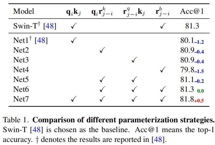
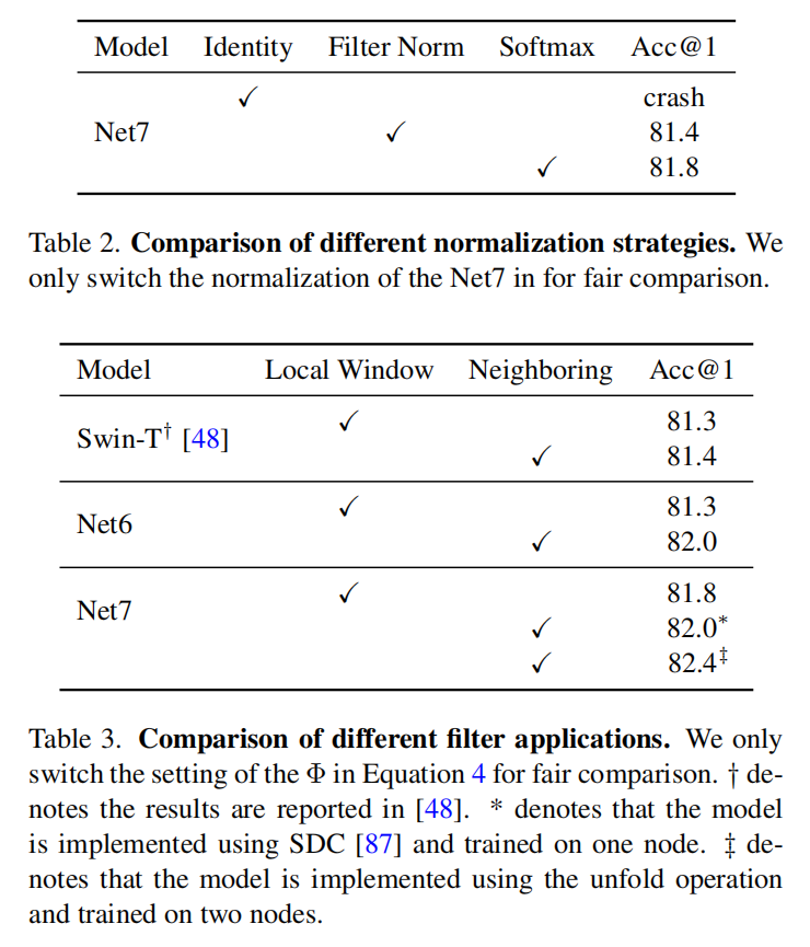
作者将以上三种结构统一到了统一范式中，对三种结构在 parameterization、normalization 和 filter application 三方面进行了对比研究，发现 relative position embedding 和 neighboring filter application 是影响表现的关键因素==如何影响？==

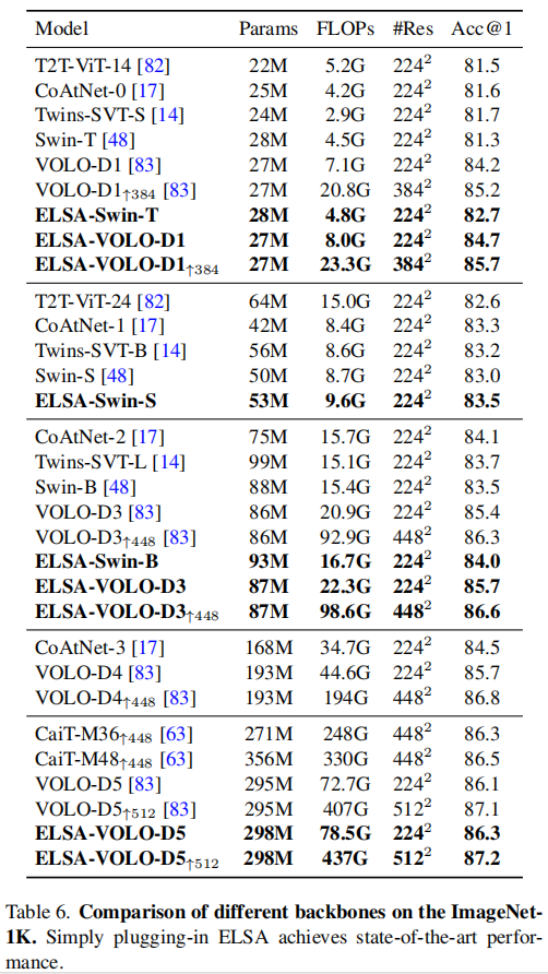
在这些发现的基础之上，作者提出了 Enhanced Local Self Attention，引入了 Hadamard attention 和 ghost head，可以用来替换 Swin-Transformer 或 VOLO 模型中的 LSA 模块

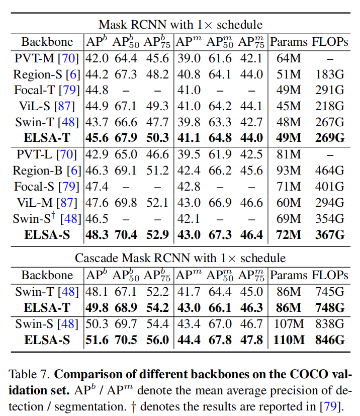
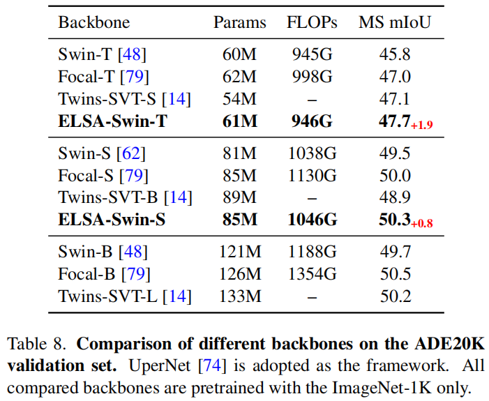
作者使用 ELSA-Swin 等网络在上下游任务进行了广泛的实验验证，其结果在基线水平上都有了一定提升。

However, calculating the dot product of queries and keys in the neighboring case is not computational-friendly. An effificient way of fifilter generation in the neighboring case is needed to replace the dot product while maintaining performance.

这句也没懂。

We compare two versions of Swin

T [48] under the same hyperparameters, and only modify

the head setting each time. Setting 1 means that the number

of heads is set to 1 for all layers. Setting 1× represents the

original setting of Swin-T, that is, the head numbers of four

stages are set to {3,6,12,24}. Setting 2× means to double

the original setting, i.e., {6,12,24,48}. Setting C denotes

that the number of heads is set to the number of channels

for all layers.

其实这个实验没有算做完，但是增加 LSA 的通道数做不下去了，因为显存不够。

Spacial Processing¶

卷积/Depth-wise Conv¶

\[ \mathbf{x}'_{i}=\sum_{j \in \Theta} \mathbf{w}_{j-i} \mathbf{x}_{j} \]

\(j\)不是一般用来代表一维数组下标吗，这里用来代表二维合适吗

Dynamic Filters¶

\[ \mathbf{x}'_{i}=\sum_{j \in \Theta} \operatorname{Norm}\left(\mathbf{x}_{i} \mathbf{w}\right) \mathbf{x}_{j} \]

\(\mathrm{w}\)是一个\(1\times 1\)的卷积权值；Norm 可以为任意的归一化函数，比如 indentity mapping、filter normalization 或 softmax

Local Self-attention¶

\[ \mathbf{x}'_{i}=\sum_{j \in \Omega} \operatorname{Softmax}_{j}\left(\mathbf{q}_{i} \mathbf{k}_{j}\right) \mathbf{v}_{j} \]

作者说：我全要¶

所以作者把以上三种组合起来，就成了

\[ \mathbf{x}'_{i}=\sum_{j \in \Phi} \operatorname{Norm}_{j}\left(\mathbf{q}_{i} \mathbf{k}_{j}+\mathbf{q}_{i} \mathbf{r}_{j-i}^{k}+\mathbf{r}_{j-i}^{q} \mathbf{k}_{j}+\mathbf{r}_{j-i}^{b}\right) \mathbf{v}_{j} \]

其中\(\Phi\)指邻域，Norm 是一种归一化操作，\(r^k_{j-i}\)和\(r^q_{j-i}\)是相对位置编码，\(r^b_{j-1}\)是相对位置偏置。

对于 DwConv，只使用\(r^b_{j-1}\)作为参数，将\(\Phi\)设置为\(\Theta\)，也就是邻域

对于 Dynamic Filter，使用\(q_ir^k_{j-i}\)作为参数

对于 LSA，使用\(q_ik_i\)作为参数，将\(\Phi\)设置为窗口

整个公式一功能有三个地方可调：\(\Phi\)、\(\text{Norm}\)和括号里要哪些不要哪些

基于以上，作者将 Swin Transformer 作为 baseline，提出了七种网络

在 Experiments 阶段作者讨论的都是自己做了什么工作，主要是解释上边几张表。

讨论¶

关键因素¶

作者认为让 LSA 平凡的原因有两点：

没有 relative position embedding，主要是 net 5 6 7
没有 filter application，局部的比全局的好

局部窗口和邻域¶

作者实验的结论是局部窗口比邻域的性能差。并且局部窗口，像 Swin 中的，需要 Swin 层成对出现。

但邻域的缺点是：吞吐量小，原因是==是否强加因果?==在 sliding neighbors 中计算\(q\)和\(k\)的点乘并不容易，需要 sliding chuck、unfold operations、以及特殊的 CUDA 算子，程序设计很难，运行的时空成本也很大。

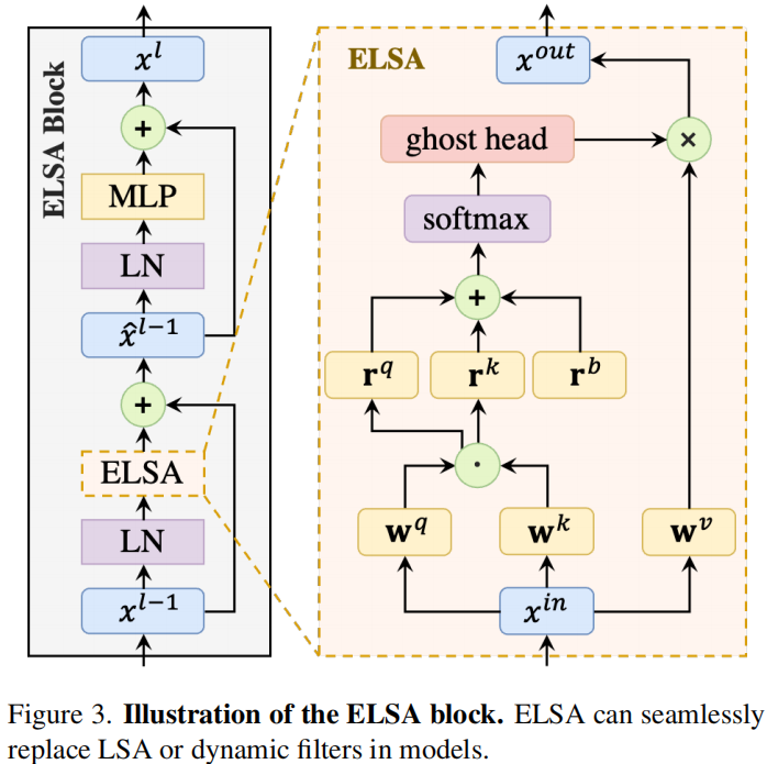
ELSA¶

基于以上实验结果，作者提出了一种新型的 LSA 模块：ELSA。关键技术是 Hadamard attention 和 ghost head module.

\[ \mathbf{x}'_{i}=\sum_{j \in \Theta} \mathrm{G}\left(\mathbf{h}_{j-i}\right) \mathbf{v}_{j} \]

其中\(\mathbf{h}\)表示 Hadamard attention 的值，\(\mathrm G(\cdot)\)表示 Ghost Attention.

\[ \mathbf{h}_{j-i}=\operatorname{Softmax}_{j}\left(\left(\mathbf{q}_{i} \odot \mathbf{k}_{i}\right) \mathbf{r}_{j-i}^{k}+\mathbf{r}_{j-i}^{q}\left(\mathbf{q}_{j} \odot \mathbf{k}_{j}\right)+\mathbf{r}_{j-i}^{b}\right) \]

定义设 \(A, B \in \mathbb{C}^{m \times n}\) 且 \(A=\left\{a_{i j}\right\}, B=\left\{b_{i j}\right\}\) ，称 \(m \times n\) 矩阵

\[ \left[\begin{array}{cccc} a_{11} b_{11} & a_{12} b_{12} & \cdots & a_{1 n} b_{1 n} \\ a_{21} b_{21} & a_{22} b_{22} & \cdots & a_{2 n} b_{2 n} \\ \vdots & \vdots & & \vdots \\ a_{m 1} b_{m 1} & a_{m 2} b_{m 2} & \cdots & a_{m n} b_{m n} \end{array}\right] \]

为矩阵 \(\mathrm{A}\) 与 \(\mathrm{B}\) 的哈达玛(Hadamard)积，记作 \(A \odot B\) 。

\[ \hat{h}_{j-i}^{c}=\operatorname{Pow}\left(o_{j-i}^{c}, \lambda\right) h_{j-i}^{c^{\prime}}+\gamma s_{j-i}^{c} \]

计算复杂度：\(O\left(n_{c} \times k s \times k s \times n_{p}\right)\)

# B: batch size, C: channel size
# N: the number of pixels
# H: the number of heads, K: kernel size
# h_attn: Hadamard attention with size (B, H, N, K*K) # lambda, gamma: hyperparameters
def init()
    mul_matrix = nn.Parameters(torch.randn(C, K, K))
    add_matrix = nn.Parameters(torch.zeros(C, K, K))
    trunc_normal_(add_matrix, std=0.02)
def ghost_head(h_attn):
    # change the size of h_attn to (B, 1, H, N, K*K)
    h_attn = h_attn.unsqueeze(1)
    # reshape the size of matrices
    mul_matrix = mul_matrix.reshape(1, C//H, H, 1, K*K)
    add_matrix = add_matrix.reshape(1, C//H, H, 1, K*K)
    # Equation 8
    h_attn = (mul_matrix ** lambda) * h_attn + gamma * add_matrix
    return h_attn.reshape(B, C, N, K*K)

结果¶

下游任务：

当然，这篇文章在写作上有许多的问题

英文表达太不地道
逻辑因果不明显，甚至有刻意模糊因果的嫌疑
数学公式使用符号太过随意，不正式，给读者的理解增加了难度
前一段研究和后一段实验的联系，过渡不自然

这篇文章也引出了一些问题：

如何提高 LSA 的效果
LSA 到底学到了什么

最后更新: 2023-01-31